Absorbed irradiance by sunlit and shaded leaf fractions

Let’s state first the following two assumptions (Goudriaan, 1977; 1988; 1994; 2016):

1. Sunlit leaves receive solar irradiance that comes from the sun (solar beam, \(I_{direct}\)),

   from the sky and/or clouds (sky-diffused, \(I_{diffuse}\)), and from leaves

   (leaf-scattered, \(I_{scattered}\)).

2. Shaded leaves do not receive the direct irradiance but do receive diffuse and scattered irradiance.

Fig. 8 Irradiance components that are absorbed by sunlit and shaded leaves. \(I_{direct} \ [W \cdot m^{-2}_{leaf}]\) is solar direct (beam) irradiance, \(I_{diffuse} \ [W \cdot m^{-2}_{leaf}]\) is sky-diffused irradiance, and \(I_{scattered} \ [W \cdot m^{-2}_{leaf}]\) is leaf-scattered irradiance.

You may have noticed in Fig. 8 that the size of the yellow arrows changes with leaf orientation. I tried by doing so to illustrate how leaf orientation affects its scattering to the incident irradiance and by that, to indicate that also the quantity of the direct irradiance absorbed by a given leaf depends on the angle between that leaf and the solar beam. For instance, the higher the sun is in the sky (time-dependent), the more likely for solar beam to reach deeper leaves inside the canopy. Furthermore, the more uniformly distributed leaf angles are (structure-dependent), the more irradiance they are likely to intercept irradiance. This interplay between the solar position and leaf angles is captured through the extinction coefficient of the direct irradiance as we will see below (extinction_and_reflectance_coefficients).

Generally, it is assumed that leaf angles through the canopy follow a uniform distribution. This means that if we took all leaves and organized them on a surface, this surface will be a hemisphere. The consequence of this assumption is that the surface of leaves that intercepts the incoming irradiance will remain the same independently from the incident angle (Fig. 9).

Fig. 9 Effect of the distribution of leaf angles on the interception to solar irradiance (after Goudriaan and van Laar, 1994). \(\beta \ [-]\) is the angle of the solar elevation.

Yet, it is more realistic to consider that leaves have a preferential declination angle (for instance, grapevine is said to have its leaves declined by 45° below the horizon). In this latter case leaves intercept different fractions of incident irradiance depending on the angle between the solar beam and leaves.

Finally, before going into equations, recall that the absorbed irradiance per unit ground area is the product of the absorbed irradiance per unit leaf area and leaf area index (leaf area per unit ground area) for each leaf fraction (sunlit and shaded). Keep in mind also that at the exception of the flux density of direct irradiance (\(I_{direct} \ [W \cdot m^{-2}{leaf}]\)), leaf area fractions and irradiance flux densities vary exponentially with depth (Fig. 10). \(I_{direct}\) is indeed constant with depth. To simply understand this fact, check sunflecks inside a canopy: all light spots shine with the same intensity throughout depth, yet, the surface of these spots reduces strongly with depth (Fig. 11).

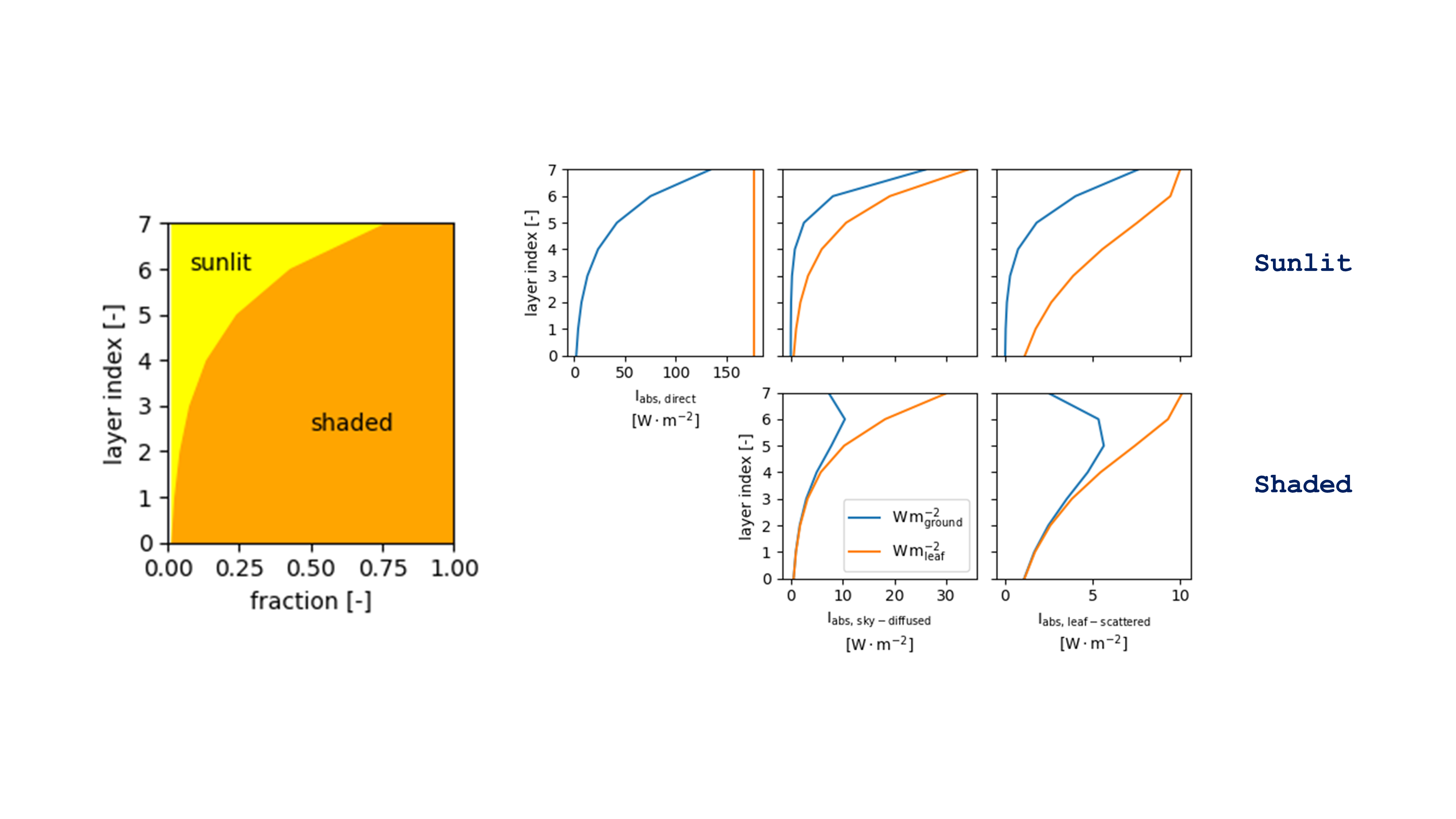
Fig. 10 Leaf fractions and irradiance intensities considered for calculating irradiance absorption by sunlit-shaded canopies. Simulations are performed for a canopy composed of 8 leaf layers having each an area thickness of \(1 \ [m^2_{leaf} \cdot m^{-2}_{ground}]\). \(I_{abs, \ direct} \ [W \cdot m^{-2}_{leaf}]\) is flux density of the absorbed direct (solar beam) irradiance, \(I_{abs, \ diffuse} \ [W \cdot m^{-2}_{leaf}]\) is flux density of the absorbed sky-diffused irradiance, and \(I_{abs, \ scattered} \ [W \cdot m^{-2}_{leaf}]\) is flux density of the absorbed leaf-scattered irradiance.

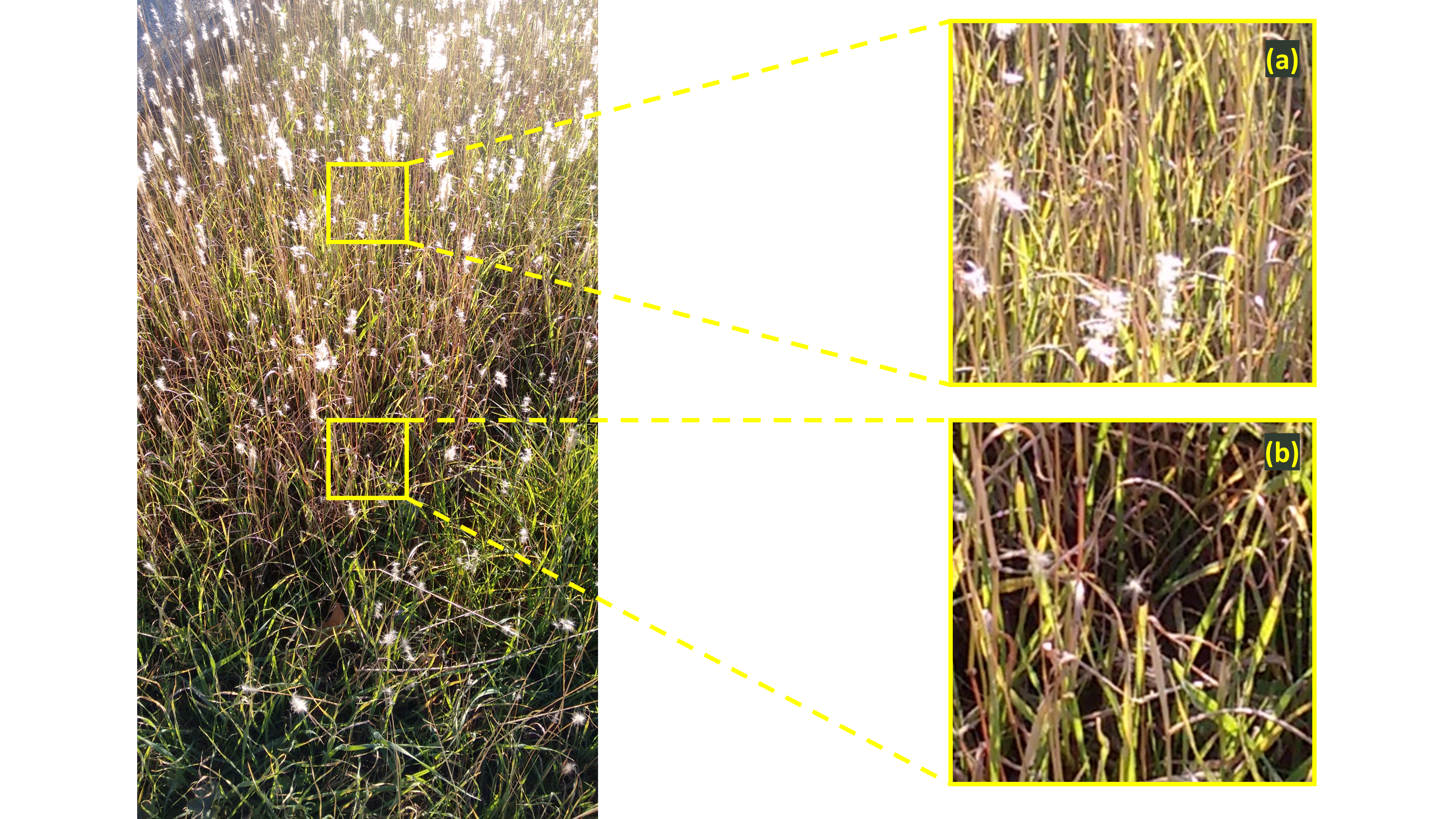
Fig. 11 The surface of sunlit leaves, not light intensity, reduces strongly with depth inside the canopy from upper \((a)\) to lower \((b)\) levels.

Extinction and reflectance coefficients

The incident direct (\(I_{inc, \ direct}\)) and sky-diffused (\(I_{inc, \ diffuse}\)) irradiacne fluxes have distinct extinction coefficients inside the canopy.

The extinction coefficient of the direct irradiance (\(k_{direct} \ [m^2_{ground} \cdot m^{-2}_{leaf}]\)) varies within the day as a function of the position of the sun (recall that the higher the sun is, the deeper sunflcks go inside the canopy). It is given as (Cowan, 1968; Goudriaan, 1977, Weiss et al., 2004, Campbell and Norman, 2012):

(9)\[k_{direct} = k_{direct, \ black} \cdot \sqrt{1 - \sigma}\]

with

(10)\[\sigma = \rho + \tau\]

and

(11)\[k_{direct, \ black} = C \cdot \frac{\bar{o}(\beta)}{\sin{\beta}}\]

where \(C \ [-]\) is the clumping factor, \(\bar{o}(\beta)\) is a projection function describing the surface of canopy elements that intercept the solar beam, \(k_{direct, \ black} \ [m^2_{ground} \cdot m^{-2}_{leaf}]\) is the extinction coefficient of black leaves and \(\sigma \ [-]\) is the leaf scattering coefficient, equal to the sum of leaf reflectance (\(\rho \ [-]\)) and transmittance (\(\tau \ [-]\)), all in the same irradiance band:

The distribution function \(\bar{o}(\beta)\) can be approximated by an ellipsoidal function following Campbell (1986) which yields:

(12)\[k_{direct, \ black} = C \cdot \frac{\sqrt{\chi ^2 + \cot^2{\beta}}}{\chi + 1.774 \cdot \left(\chi + 1.182\right) ^{-0.733}}\]

where \(\chi \ [-]\) is the eccentricity of the ellipsoid, calculated as a function of the leaf characteristic angle \(\bar{\alpha}\) following Campbell (1990) as:

(13)\[\chi = \left(\frac{\bar{\alpha}}{9.65} \right) ^ {-0.6061} - 3\]

It is noteworthy that when \(\alpha = 56 ^\circ\) then \(\chi = 1\) and the ellipsoidal distribution becomes a spherical distribution.

The extinction coefficient of the sky-diffused irradiance (\(k_{diffuse} \ [m^2_{ground} \cdot m^{-2}_{leaf}]\)) is independent from sun’s position but varies with the total leaf area of the canopy. \(k_{diffuse}\) is derived using (9) by considering the sky as an ensemble of finite sectors that send, each, diffuse irradiance as if it were a beam irradiance. These sectors may be represented by rings. The extinction coefficient \(k_{diffuse}\) is given as:

(14)\[k_{diffuse} = - \frac{1}{L_t} \cdot \ln \left( \Sigma_i^n { \left( c_i \cdot e ^ {- k_{direct}(\beta_{sky, \ i}) \cdot L_t} \right) } \right)\]

where \(L_t \ [m^2_{leaf} \ m^{-2}_{ground}]\) is the canopy total leaf area index, \(\beta_{sky, \ i} \ [-]\) is the angle elevation of each sky ring, \(c_i \ [-]\) is a weighing factor accounting for the relative surface area of each sky ring, and \(n \ [-]\) is the number of sky rings that form the sky dome.

Goudriaan (1988) showed that \(k_{diffuse}\) can be adequately estimated as long as the number of sky rings is greater or equal to 3. Thus for 3 rings spanning respectively over angular sectors with an increasing angle of 30 \(^\circ\) (\(\left[ 0, \frac{\pi}{6} \right]\), \(\left[ \frac{\pi}{6}, \frac{\pi}{3} \right]\), \(\left[ \frac{\pi}{3}, \frac{\pi}{2} \right]\)) the last equation becomes:

(15)\[\begin{split}k_{diffuse} = - \frac{1}{L_t} \cdot \ln \left( \begin{array}{1} 0.178 \cdot e^ {- k_{direct}(\frac{\pi}{12}) \cdot L_t} \\ + 0.514 \cdot e^ {- k_{direct}(\frac{3\pi}{12}) \cdot L_t} \\ + 0.308 \cdot e^ {- k_{direct}(\frac{5\pi}{12}) \cdot L_t} \end{array} \right)\end{split}\]

where the coefficients 0.178, 0.514 and 0.308 are calculated for a standard sky over cast (SOC) assuming a ration 3:1 between zenith and minimum horizontal sky illuminance.

Reflectance coefficients to direct and diffuse irradiance are needed in absorbed irradiance calculations (cf. irradiance_absorption).

Canopy reflectance to direct irradiance \(\rho_{direct} \ [-]\) depends on leaf angles distribution and the declination of the solar beam. \(\rho_{direct}\) is lowest when the sun is closest the zenith and highest as solar inclination approaches 0 \(^\circ\) (sun is grazing over horizontal leaves). \(\rho_{dir}\) is given by Goudriaan (1977) as:

(16)\[\rho_{direct} = 1 - \exp {\left( - \frac{2 \cdot \rho_h \cdot k_{direct, \ black}}{1 + k_{direct, \ black}} \right)}\]

where \(\rho_h \ [-]\) is the reflection coefficient of a canopy having horizontal leaves, defined as:

(17)\[\rho_h = \frac{1 - \sqrt{1 - \sigma}}{1 + \sqrt{1 - \sigma}}\]

Canopy reflectance coefficient to the sky-diffused irradiance (\(\rho_{diffuse} \ [m^2_{ground} \cdot m^{-2}_{leaf}]\)) is farely constant across canopies and its value can roughly be set to 0.057 for the photosynthetically active radiation (PAR) band and 0.389 for the near infrared (NIR) band (Goudriaan and van Laar, 1994).

Irradiance absorption

Let’s recall first that sunlit leaves absorbe irradiance that comes from the solar beam (\(I_{abs, \ direct} \ [W \cdot m^{-2}_{leaf}]\)), sky-diffused (\(I_{abs, \ sky-diffused} \ [W \cdot m^{-2}_{leaf}]\)), and leaf-scattered (\(I_{abs, \ leaf-scattered} \ [W \cdot m^{-2}_{leaf}]\)) irradiance. Shaded leaves receive only sky-diffused and leaf-scattered irradiance (cf. absorbed_sunlit_shaded).

On a ground area basis, irradiance absorption by sunlit \(I_{abs, \ sunlit} \ [W \cdot m^{-2}_{ground}]\) and shaded \(I_{abs, \ shaded} \ [W \cdot m^{-2}_{ground}]\) leaf fractions of a leaf layer spanning between depths \(L_u \ [m^2_{leaf} \cdot m^{-2}_{ground}]\) and \(L_l \ [m^2_{leaf} \cdot m^{-2}_{ground}]\) are given as:

(18)\[I_{abs, \ sunlit} = \int_{L_u}^{L_l} { \left( I_{abs, \ direct} + I_{abs, \ sky-diffused} + I_{abs, \ leaf-scattered} \right) \cdot \phi_{sunlit} \ dL }\]

(19)\[I_{abs, \ sunlit} = \int_{L_u}^{L_l} { \left( I_{abs, \ sky-diffused} + I_{abs, \ leaf-scattered} \right) \cdot \phi_{shaded} \ dL }\]

where \(\phi_{sunlit} \ [m^2_{leaf} \cdot m^{-2}_{leaf}]\) and \(\phi_{shaded} \ [m^2_{leaf} \cdot m^{-2}_{leaf}]\) are respectively leaf fractions of sunlit and shaded leaves, given as:

(20)\[\phi_{sunlit} = e ^ {- k_{direct, \ black} \cdot L}\]

(21)\[\phi_{shaded} = 1 - \phi_{sunlit}\]

\(I_{abs, \ direct}\), \(I_{abs, \ sky-diffused}\) and \(I_{abs, \ leaf-scattered}\) are given in the three following equations, respectively:

(22)\[ \begin{align}\begin{aligned}\begin{array}\\\begin{split} I_{abs, \ direct} &= I_{inc, \ direct} \cdot (1 - \sigma) \cdot k_{direct, \ black} \\ I_{abs, \ sky-diffused} &= I_{inc, \ diffuse} \cdot \left( 1 - \rho_{diffuse} \right) \cdot k_{diffuse} \cdot e ^ {- k_{diffuse} \cdot L } \\ I_{abs, \ leaf_scattered} &= I_{inc, \ direct} \cdot \left[ \begin{array} ((1 - \rho_{direct}) \cdot k_{direct} e ^ {-k_{diffuse} \cdot L} \\ - (1 - \sigma) \cdot k_{direct, \ black} \cdot e ^ {-k_{direct, \ black} \cdot L} \end{array} \right]\end{split}\\\end{array}\end{aligned}\end{align} \]

where \(I_{inc, \ direct}\) and \(I_{inc, \ diffuse} \ [W \ m^{-2}_{ground}]\) are the incident direct and sky-diffused irradiance, respectively.

Layered canopies

For a leaf layer spanning between depths \(L_u \ [m^2_{leaf} \cdot m^{-2}_{ground}]\) and \(L_l \ [m^2_{leaf} \cdot m^{-2}_{ground}]\) equations (18) and (19) become:

(23)\[\begin{split}I_{abs, \ sunlit} & = I_{inc, \ direct} \cdot (1 - \sigma) \cdot \left( e ^ {- k_{direct, \ black} \cdot L_u} - e ^ {- k_{direct, \ black} \cdot L_l} \right) \\ & + I_{inc, \ diffuse} \cdot \left( 1 - \rho_{diffuse} \right) \cdot \frac{k_{diffuse}}{k_{diffuse} + k_{direct, \ black}} \cdot \left( \begin{array} + e ^ {- (k_{diffuse} + k_{direct, \ black}) \cdot L_u } \\ - e ^ {- (k_{diffuse} + k_{direct, \ black}) \cdot L_l } \end{array} \right) \\ & + I_{inc, \ direct} \cdot \left[ \begin{array}{1} \left( 1 - \rho_{direct} \right) \cdot \frac{k_{direct}}{k_{direct} + k_{direct, \ black}} \cdot \left( \begin{array} + e ^ {- (k_{direct} + k_{direct, \ black}) \cdot L_u } \\ - e ^ {- (k_{direct} + k_{direct, \ black}) \cdot L_l } \end{array} \right) \\ - (1 - \sigma) \cdot \frac{1}{2} \cdot \left( e ^ {- 2 \cdot k_{direct, \ black} \cdot L_u } - e ^ {-2 \cdot k_{direct, \ black} \cdot L_l } \right) \end{array} \right]\end{split}\]

(24)\[\begin{split}I_{abs, \ shaded} & = I_{inc, \ diffuse} \cdot \left( 1 - \rho_{diffuse} \right) \cdot \left( \begin{array}{1} \left( \begin{array} + e ^ {- k_{diffuse} \cdot L_u } \\ - e ^ {- k_{diffuse} \cdot L_l } \end{array} \right) \\ - \frac{k_{diffuse}}{k_{diffuse} + k_{direct, \ black}} \cdot \left( \begin{array} + e ^ {- (k_{diffuse} + k_{direct, \ black}) \cdot L_u } \\ - e ^ {- (k_{diffuse} + k_{direct, \ black}) \cdot L_l } \end{array} \right) \end{array} \right) \\ & + I_{inc, \ direct} \cdot \left[ \begin{array}{1} \left( 1 - \rho_{direct} \right) \cdot \left( \begin{array}{1} \left( \begin{array} + e ^ {- k_{direct} \cdot L_u } \\ - e ^ {- k_{direct} \cdot L_l } \end{array} \right) \\ - \frac{k_{direct}}{k_{direct} + k_{direct, \ black}} \cdot \left( \begin{array} + e ^ {- (k_{direct} + k_{direct, \ black}) \cdot L_u } \\ - e ^ {- (k_{direct} + k_{direct, \ black}) \cdot L_l } \end{array} \right) \end{array} \right) \\ - (1 - \sigma) \cdot \left( \begin{array}{1} \left( e ^ {- k_{direct, \ black} \cdot L_u } - e ^ {- k_{direct, \ black} \cdot L_l } \right) \\ - \frac{1}{2} \cdot \left( e ^ {- 2 \cdot k_{direct, \ black} \cdot L_u } - e ^ {-2 \cdot k_{direct, \ black} \cdot L_l } \right) \end{array} \right) \end{array} \right]\end{split}\]

Bigleaf canopies

For a bigleaf canopy equations (23) and (24) become respectively:

(25)\[\begin{split}I_{abs, \ sunlit} & = I_{inc, \ direct} \cdot (1 - \sigma) \cdot \left( 1 - e ^ {- k_{direct, \ black} \cdot L_t} \right) \\ & + I_{inc, \ diffuse} \cdot \left( 1 - \rho_{diffuse} \right) \cdot \frac{k_{diffuse}}{k_{diffuse} + k_{direct, \ black}} \cdot \left( \begin{array} + 1 - e ^ {- (k_{diffuse} + k_{direct, \ black}) \cdot L_t } \end{array} \right) \\ & + I_{inc, \ direct} \cdot \left[ \begin{array}{1} \left( 1 - \rho_{direct} \right) \cdot \frac{k_{direct}}{k_{direct} + k_{direct, \ black}} \cdot \left( \begin{array} + 1 - e ^ {- (k_{direct} + k_{direct, \ black}) \cdot L_t } \end{array} \right) \\ - (1 - \sigma) \cdot \frac{1}{2} \cdot \left( 1 - e ^ {-2 \cdot k_{direct, \ black} \cdot L_t } \right) \end{array} \right]\end{split}\]

(26)\[\begin{split}I_{abs, \ shaded} & = I_{inc, \ diffuse} \cdot \left( 1 - \rho_{diffuse} \right) \cdot \left( \begin{array}{1} \left( \begin{array} + 1 - e ^ {- k_{diffuse} \cdot L_t } \end{array} \right) \\ - \frac{k_{diffuse}}{k_{diffuse} + k_{direct, \ black}} \cdot \left( \begin{array} + 1 - e ^ {- (k_{diffuse} + k_{direct, \ black}) \cdot L_t } \end{array} \right) \end{array} \right) \\ & + I_{inc, \ direct} \cdot \left[ \begin{array}{1} \left( 1 - \rho_{direct} \right) \cdot \left( \begin{array}{1} \left( \begin{array} + 1 - e ^ {- k_{direct} \cdot L_t } \end{array} \right) \\ - \frac{k_{direct}}{k_{direct} + k_{direct, \ black}} \cdot \left( \begin{array} + 1 - e ^ {- (k_{direct} + k_{direct, \ black}) \cdot L_t } \end{array} \right) \end{array} \right) \\ - (1 - \sigma) \cdot \left( \begin{array}{1} \left( 1 - e ^ {- k_{direct, \ black} \cdot L_t } \right) \\ - \frac{1}{2} \cdot \left( 1 - e ^ {-2 \cdot k_{direct, \ black} \cdot L_t } \right) \end{array} \right) \end{array} \right]\end{split}\]